
Mastering Basic Google Sheets Functions: A Comprehensive Guide
24 min read
Mastering Basic Google Sheets Functions: A Comprehensive Guide
Table of Contents
(Click to expand)
- Introduction to Google Sheets Functions
- Basic Functions for Beginners
- Intermediate Functions for Data Analysis
- IF function: Using conditional logic to categorize data
- AND/OR functions
- VLOOKUP function: Finding and retrieving data from a table
- CONCATENATE function: Combining text from different cells into one cell
- CLEAN function: Remove non-printable characters
- TRIM function: Remove leading, trailing, and repeated spaces
- Functions for Date and Time
- Advanced Functions for Complex Data Manipulation
- Tips for Maximizing Efficiency with Functions
- Common Errors and Troubleshooting Tips
- Best Practices for Organizing and Documenting Functions
- Integrating Functions with Other Google Sheets Features
- Conclusion
Unleash the full potential of Google Sheets by mastering the art of using functions. This comprehensive guide delves into the various aspects of functions in Google Sheets, providing practical tips and insights for maximum efficiency. Whether you're a beginner or a seasoned user, this article offers valuable information to help you optimize your use of functions and enhance your productivity.
Introduction to Google Sheets Functions
Google Sheets functions are powerful tools that allow users to perform various calculations, manipulate data, and automate tasks within a spreadsheet. These functions are essential for anyone working with data, whether it's for personal finance tracking, business analysis, or academic research. By mastering the art of using functions in Google Sheets, users can unlock the full potential of this versatile tool and significantly enhance their productivity.
What are the functions in Google Sheets?
In Google Sheets, functions are predefined formulas that perform specific calculations or manipulations on data. They are designed to simplify complex tasks and make it easier to work with large sets of data. Functions can range from simple arithmetic operations to advanced data analysis and manipulation.
How to use functions in Google Sheets?
To use functions in Google Sheets, start by typing an equal sign (=) in a cell, followed by the name of the function you want to use. Then, input the necessary arguments within parentheses to specify the data you want the function to operate on. For example, to sum a range of numbers, you can use the SUM function by typing =SUM(A1:A10) to add the numbers in cells A1 to A10. Additionally, you can use the autocomplete feature in Google Sheets to easily find and select the function you need, saving time and reducing the risk of errors in your formulas. By familiarizing yourself with the various functions available and understanding how to use them effectively, you can streamline your data management and analysis processes in Google Sheets.
Why are functions important for data analysis and manipulation?
Functions play a crucial role in data analysis and manipulation by providing a structured and efficient way to perform calculations and extract insights from data. They enable users to automate repetitive tasks, apply conditional logic, and retrieve specific information from a dataset. By using functions, users can save time, reduce errors, and gain valuable insights from their data.
Basic Functions for Beginners
This article provides a comprehensive overview of the essential functions of Google Sheets, a powerful tool for organizing and analyzing data. Whether you are new to spreadsheets or aiming to improve your skills, this exploration will help you learn the basic functions in Google Sheets. Google Sheets functions include a wide range of capabilities, from simple arithmetic operations to more complex data manipulation and analysis. Some of the basic functions covered in this article include SUM, AVERAGE, MAX, MIN, and COUNT. These functions are essential for performing calculations and summarizing data in your spreadsheets. Additionally, we will also explore how to use these functions in combination with other features of Google Sheets, such as conditional logic and data manipulation, to create more powerful and dynamic spreadsheets. By the end of this article, you will have a solid understanding of the basic functions in Google Sheets and how to apply them to your own data analysis and organization needs.
SUM function: Adding up numbers in a range
The SUM function is used to add up a range of numbers in a spreadsheet.
Syntax
SUM(value1, [value2, ...])
- value1 - The first number or range to add together.
- value2, ... - [ OPTIONAL ] - Additional numbers or ranges to add to value1.
Ref: SUM
Example
To add the values in cells A1 to A5, you can use the formula:
=SUM(A1:A5)
AVERAGE function: Calculating the average of a range of numbers
The AVERAGE function in Google Sheets calculates the average of a range of numbers.
Syntax
AVERAGE(value1, [value2, ...])
- value1 - The first value or range to consider when calculating the average value.
- value2, ... - [ OPTIONAL ] - Additional values or ranges to consider when calculating the average value.
Ref: AVERAGE
Example
To find the average of values in cells B1 to B5, you can use the formula:
=AVERAGE(B1:B5)
COUNT function: Counting the number of cells in a range containing numbers
The COUNT function in Google Sheets counts the number of cells in a range that contains numbers.
Syntax
COUNT(value1, [value2, ...])
- value1 - The first value or range to consider when counting.
- value2, ... - [ OPTIONAL ] - Additional values or ranges to consider when counting.
Ref: COUNT
Example
To count the number of cells with values in cells C1 to C5, you can use the formula:
=COUNT(C1:C5)
MAX/MIN functions
The MAX and MIN functions are used to find the maximum and minimum values in a range, respectively.
Syntax
MAX/MIN(value1, [value2, ...])
- value1 - The first value or range to consider when calculating the maximum/minimum value.
- value2, ... - [ OPTIONAL ] - Additional values or ranges to consider when calculating the maximum/minimum value.
Ref: MAX
Ref: MIN
Example
To find the maximum value in cells D1 to D5, you can use the formula:
=MAX(D1:D5)
Intermediate Functions for Data Analysis
IF function: Using conditional logic to categorize data
The IF function allows users to apply conditional logic to categorize data based on specified criteria. It is commonly used to assign labels or perform calculations based on certain conditions. Additionally, the IF function can be nested within other functions to create more complex conditional statements, allowing for even more advanced categorization and analysis of data. Overall, the IF function is a powerful tool for organizing and interpreting data in spreadsheets and databases.
Syntax
IF(logical_expression, value_if_true, value_if_false)
- logical_expression - An expression or reference to a cell containing an expression that represents some logical value, i.e. TRUE or FALSE.
- value_if_true - The value that the function returns if logical_expression is TRUE.
- value_if_false - [ OPTIONAL - blank by default ] - The value that the function returns if logical_expression is FALSE.
Ref: IF
Example
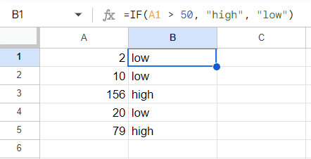
For example, the IF function can be used to categorize sales data as high, or low based on predefined sales targets. This can help users quickly analyze and understand their sales performance.
=IF(A1 > 50, "high", "low")
AND/OR functions
The AND and OR functions are used to evaluate multiple conditions and return a true or false value based on the specified criteria. The AND function in Google Sheets returns true only if all the specified conditions are true, while the OR function returns true if at least one of the specified conditions is true. These functions are commonly used in Google Sheets to perform logical operations. Understanding how to use these functions can greatly enhance your ability to analyze and manipulate data.
Syntax
AND/OR(logical_expression1, [logical_expression2, ...])
- logical_expression1 - An expression or reference to a cell containing an expression that represents some logical value, i.e. TRUE or FALSE, or an expression that can be coerced to a logical value.
- logical_expression2, … - [ OPTIONAL ] - Additional expressions or references to cells containing expressions representing some logical values, i.e. TRUE or FALSE, or expressions that can be coerced to logical values.
Ref: AND
Ref: OR
Example
AND
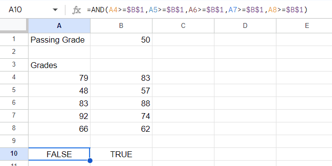
The AND function can be used to check if a student has passed all the required exams.
=AND(A4>=$B$1,A5>=$B$1,A6>=$B$1,A7>=$B$1,A8>=$B$1)
OR
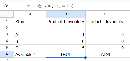
The OR function can be used to check if a product is available in at least one store.
=OR(B3,B4,B5)
VLOOKUP function: Finding and retrieving data from a table
The VLOOKUP function is used to find and retrieve specific data from a table based on a given key. It is particularly useful for searching and referencing information from a large dataset. The function takes four arguments: the lookup value, the table array, the column index number, and the exact match. It is important to ensure that the lookup value is unique in the first column of the table array for the function to work accurately. Additionally, the exact match parameter allows you to specify whether you want an exact match or an approximate match for the lookup value.
Syntax
=VLOOKUP(search_key, range, index, [is_sorted])
- search_key: The value to search for in the first column of the range.
- range: The upper and lower values to consider for the search.
- index: The index of the column with the return value of the range. The index must be a positive integer.
- is_sorted: Optional input. Choose an option:
- FALSE = Exact match. This is recommended.
- TRUE = Approximate match. This is the default if is_sorted is unspecified. Important: Before you use an approximate match, sort your search key in ascending order. Otherwise, you may likely get a wrong return value. Learn why you may encounter a wrong return value.
Ref: VLOOKUP
Example
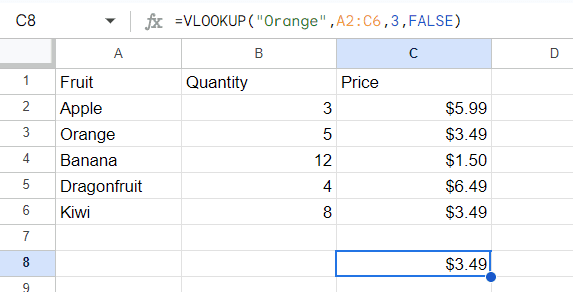
For example, you can use the VLOOKUP function to retrieve a product's price from a price list.
=VLOOKUP("Orange",A2:C6,3,FALSE)
CONCATENATE function: Combining text from different cells into one cell
The CONCATENATE function is used to combine text from different cells into a single cell. It is handy for creating custom labels or joining text values together. This can be especially useful when creating mailing labels or generating personalized reports. The syntax for the CONCATENATE function is straightforward, as you simply need to input the cell references or text strings you want to combine.
Syntax
CONCATENATE(string1, [string2, ...])
- string1 - The initial string.
- string2, ... - [ OPTIONAL ] - Additional strings to append in sequence.
Ref: CONCATENATE
Example
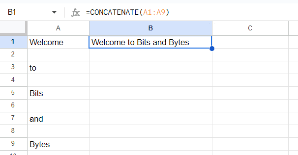
We can use the CONCATENATE function to combine the text in multiple rows.
=CONCATENATE(A1:A9)
CLEAN function: Remove non-printable characters
The CLEAN function is another useful tool in Google Sheets that is used to remove non-printable characters from text. This function is particularly helpful when dealing with data that may have been imported from external sources and contains unwanted non-printable characters. By using the CLEAN function, users can ensure that their data is free from any hidden characters that could potentially cause issues with formatting or data manipulation.
Syntax
CLEAN(text)
- text - The text whose non-printable characters are to be removed.
Ref: CLEAN
Example
=CLEAN(A1)
TRIM function: Remove leading, trailing, and repeated spaces
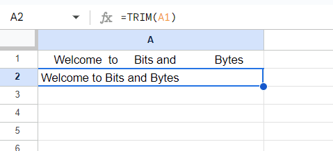
The TRIM function is a valuable tool for removing leading, trailing, and repeated spaces from text. This is especially important when working with data that may have been copied or imported from other sources, as extra spaces can affect the accuracy of calculations and sorting. By using the TRIM function, users can ensure that their data is clean and consistent, improving the overall quality of their spreadsheets.
Syntax
TRIM(text)
- text - The string or reference to a cell containing a string to be trimmed.
Ref: TRIM
Example
=TRIM(A1)
Functions for Date and Time
TODAY function
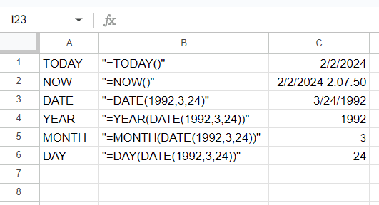
The TODAY function in Google Sheets returns the current date in a selected cell. It is useful for tracking the current date in a spreadsheet. This function is particularly handy for creating dynamic timestamps in your spreadsheet, ensuring that the date is always up to date without the need for manual updates. Additionally, the TODAY function can be combined with other functions to perform various date calculations, such as determining the number of days between two dates or automatically updating deadlines based on the current date. By utilizing the TODAY function, you can streamline your spreadsheet processes and ensure accurate and timely date tracking for your data analysis and reporting needs.
Syntax
TODAY()
Ref: TODAY
NOW function
The NOW function returns the current date and time in a selected cell. It helps track the current date and time in a spreadsheet. The NOW function is particularly useful for time-sensitive calculations and for creating dynamic reports that automatically update with the current date and time. For example, you can use the NOW function to timestamp when data was last updated, to calculate the age of a person or an item based on the current date, or to track the time elapsed since a specific event. Additionally, the NOW function can be combined with other functions, such as IF or conditional formatting, to create alerts or reminders based on the current date and time. This can be especially helpful in project management or scheduling tasks within a spreadsheet. Overall, the NOW function provides a convenient way to incorporate real-time data and time-based calculations into your spreadsheets, enhancing their accuracy and relevance.
Syntax
NOW()
Ref: NOW
DATE function
The DATE function in Google Sheets allows users to create a date based on specified year, month, and day values. This function is valuable for generating specific dates for various purposes, such as scheduling events, tracking deadlines, or calculating durations. By using the DATE function, you can ensure consistency and accuracy in your date-related data, as well as facilitate date-based calculations within your spreadsheet. Additionally, the DATE function can be combined with other functions, such as IF or conditional formatting, to automate date-related tasks and create visual cues for date ranges or upcoming events. Overall, the DATE function provides a powerful tool for managing date-related information and optimizing the functionality of your Google Sheets.
Syntax
DATE(year, month, day)
- year - The year component of the date.
- month - The month component of the date.
- day - The day component of the date.
Ref: DATE
Example
=DATE(1992,3,24)
YEAR function
The YEAR function extracts the year from a given date and returns it in the selected cell. This can be useful for analyzing data based on the year, such as sales trends or financial reports. To use the YEAR function, simply input the date from which you want to extract the year and the function will return the year value. This can help streamline data analysis and reporting processes within your spreadsheet. Additionally, the YEAR function can be combined with other functions to perform more complex date and time calculations, providing flexibility and efficiency in your data management tasks.
Syntax
YEAR(date)
- date - The date from which to calculate the year. Must be a cell reference to a cell containing a date, a function returning a date type, or a number.
Ref: YEAR
Example
=YEAR(DATE(1992,3,24))
MONTH function
The MONTH function is another useful tool for extracting specific information from a date. It returns the month from a given date and displays it in the selected cell. This can be valuable for organizing data by month, such as tracking monthly expenses or analyzing seasonal trends. Similar to the YEAR function, the MONTH function can be combined with other functions to perform more advanced date and time calculations, enhancing the capabilities of your spreadsheet. By utilizing the MONTH function, you can efficiently manage and analyze date-related information, improving the accuracy and effectiveness of your data analysis processes.
Syntax
MONTH(date)
- date - The date from which to extract the month. Must be a reference to a cell containing a date, a function returning a date type or a number.
Ref: MONTH
Example
=MONTH(DATE(1992,3,24))
DAY function
The DAY function is designed to extract the day from a given date and display it in the selected cell. This can be beneficial for tasks such as tracking the frequency of certain events or analyzing daily patterns. By incorporating the DAY function into your spreadsheet, you can enhance your ability to organize and interpret date-related data, contributing to more informed decision-making. Additionally, the DAY function can be combined with other functions to perform complex date and time calculations, allowing for greater flexibility and efficiency in managing and analyzing your data. With the inclusion of the DAY function, you can further optimize your spreadsheet for comprehensive date and time analysis, empowering you to derive valuable insights from your data.
Syntax
DAY(date)
- date - The date from which to extract the day. Must be a reference to a cell containing a date, a function returning a date type, or a number.
Ref: DAY
Example
=DAY(DATE(1992,3,24))
Advanced Functions for Complex Data Manipulation
QUERY function: Extracting specific data from a large dataset
The Google Sheets QUERY function is a powerful tool for extracting specific data from a large dataset based on specified criteria. It allows users to filter, sort, and manipulate data with SQL-like language called the Google Visualization API Query Language. For example, the QUERY function can be used to extract only the sales data from a specific region or to filter out any records that do not meet certain criteria. This can be especially useful when dealing with large datasets where manually sorting through the information would be time-consuming and prone to errors. By using the QUERY function, users can efficiently retrieve the exact data they need for analysis or reporting purposes, saving time and ensuring accuracy. Additionally, the function can also be used to perform calculations and aggregate functions on the extracted data, providing further flexibility and insight into the dataset.
Syntax
QUERY(data, query, [headers])
- data - The range of cells to perform the query on.
- query - The query to perform, written in the Google Visualization API Query Language.
- headers - [ OPTIONAL ] - The number of header rows at the top of data. If omitted or set to -1, the value is guessed based on the content of data.
Ref: QUERY
SPLIT function
The SPLIT function is used to split text into separate cells based on a specified delimiter. It is handy for separating text values into individual components. This can be particularly useful when cleaning and organizing data for further analysis or reporting.
Syntax
SPLIT(text, delimiter, [split_by_each], [remove_empty_text])
- text - The text to divide.
- delimiter - The character or characters to use to split text.
- split_by_each - [ OPTIONAL - TRUE by default ] - Whether or not to divide text around each character contained in delimiter.
- remove_empty_text - [ OPTIONAL - TRUE by default ] - Whether or not to remove empty text messages from the split results.
Ref: SPLIT
Example
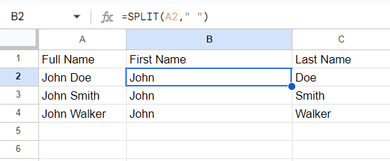
For example, if you have a column containing full names, you can use the SPLIT function to separate the first and last names into separate cells.
=SPLIT(A2," ")
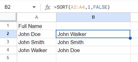
SORT function
The SORT function is used to sort the rows of a range based on the values in one or more columns. It is particularly useful for organizing and arranging data in a specific order. This can make it easier to identify trends or outliers within the dataset. Additionally, the SORT function allows for the sorting of data in ascending or descending order, providing further control over how the information is presented. By using the SORT function, users can quickly and efficiently organize their data to meet their specific needs, improving the overall usability and readability of the dataset.
Syntax
SORT(range, sort_column, is_ascending, [sort_column2, is_ascending2, ...])
- range - The data to be sorted.
- sort_column - The index of the column in range or a range outside of range containing the values by which to sort. A range specified as a sort_column must be a single column with the same number of rows as range.
- is_ascending - TRUE or FALSE indicating whether to sort sort_column in ascending order. FALSE sorts in descending order.
- sort_column2, is_ascending2, ... - [ OPTIONAL ] - Additional columns and sort order flags beyond the first, in order of precedence.
Ref: SORT
Example
For example, the SORT function can be used to arrange a list of names alphabetically.
=SORT(A2:A4,1,FALSE)
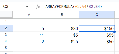
ARRAYFORMULA function: Applying a formula to an entire column or range
The ARRAYFORMULA function allows users to apply a formula to an entire column or range, eliminating the need to drag the formula down manually. This can be particularly useful when working with large datasets or when needing to apply the same formula to multiple rows of data. By using the ARRAYFORMULA function, users can streamline their workflow and ensure consistency in calculations across the dataset. Additionally, this function can help reduce the potential for errors that may arise from manually applying formulas to individual cells. Overall, the ARRAYFORMULA function is a valuable tool for efficiently applying formulas to large datasets and maintaining accuracy and consistency in data analysis and reporting.
Syntax
ARRAYFORMULA(array_formula)
- array_formula - A range, mathematical expression using one cell range or multiple ranges of the same size, or a function that returns a result greater than one cell.
Ref: ARRAYFORMULA
Example
ARRAYFORMULA can be used to do calculations for an entire column.
=ARRAYFORMULA(A2:A4*B2:B4)
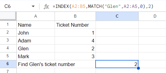
INDEX and MATCH functions: Looking up and retrieving data from a table
The INDEX and MATCH functions are often used together to look up and retrieve data from a table based on specified criteria. They provide a flexible and powerful way to search for information within a dataset.
Syntax
INDEX
INDEX(reference, [row], [column])
- reference - The range of cells from which the values are returned.
- row - [OPTIONAL - 0 by default] - The index of the row to be returned from within the reference range of cells.
- column - [OPTIONAL - 0 by default] - The index of the column to be returned from within the reference range of cells.
Ref: INDEX
MATCH
MATCH(search_key, range, [search_type])
- search_key - The value to search for. For example, 42, "Cats", or I24.
- range - The one-dimensional array to be searched. If a range with both height and width greater than 1 is used, MATCH will return #N/A!.
- search_type - [ OPTIONAL - 1 by default ] - The manner in which to search.
- 1, the default, causes MATCH to assume that the range is sorted in ascending order and return the largest value less than or equal to search_key.
- 0 indicates exact match, and is required in situations where range is not sorted.
- -1 causes MATCH to assume that the range is sorted in descending order and return the smallest value greater than or equal to search_key.
Ref: MATCH
Example
For example, we can use the combination of the INDEX and the MATCH function to find a person's ticket number.
=INDEX(A2:B5,MATCH("Glen",A2:A5,0),2)
Tips for Maximizing Efficiency with Functions
Referencing the official Google Sheets functions list
When in doubt, refer to the Google Sheets functions list for clarification or to learn about other functions.
Using named ranges to simplify function usage
Named ranges can simplify function usage by assigning a name to a specific range of cells. This makes it easier to reference the range in functions and formulas.
Utilizing the "Insert Function" feature for quick access to functions
The "Insert Function" feature in Google Sheets provides quick access to a list of functions and their descriptions, making it easier to find and use the right function for a specific task.
Understanding and using function arguments effectively
Function arguments are the input values that a function uses to perform a calculation or manipulation. Understanding how to use function arguments effectively can enhance the efficiency and accuracy of functions.
Common Errors and Troubleshooting Tips
DIV/0! error: Dividing by zero in a function
The #DIV/0! error occurs when a function attempts to divide a value by zero. To avoid this error, users should ensure that the divisor is not zero or use an IF statement to handle zero values.
VALUE! error: Incorrect data type used in a function
The #VALUE! error occurs when a function receives an incorrect data type as an argument. Users should verify that the input values are of the correct data type to prevent this error.
REF! error: Referencing a cell that is not valid
The #REF! error occurs when a function references a cell that is not valid, such as a deleted cell or a cell in a different sheet. Users should double-check their cell references to resolve this error.
Best Practices for Organizing and Documenting Functions
Using comments to explain the purpose of functions
Adding comments to functions can help users document the purpose and usage of each function, making it easier to understand and maintain the spreadsheet.
Grouping related functions together for easier management
Grouping related functions together in a spreadsheet can streamline the organization and management of functions, especially in complex datasets.
Creating a separate sheet for documenting and explaining complex functions
For complex functions or formulas, creating a separate sheet to document and explain their usage can provide a clear reference for users and collaborators.
Integrating Functions with Other Google Sheets Features
Using functions in combination with filters and sorting
Functions can be integrated with filters and sorting to perform advanced data analysis and manipulation, allowing users to extract specific information and organize data effectively.
Incorporating functions into charts and graphs for data visualization
By incorporating functions into charts and graphs, users can visualize data and gain insights into trends, patterns, and relationships within the dataset.
Collaborating with others by sharing sheets with functions
Google Sheets allows users to collaborate and share spreadsheets with others, enabling teams to work together on data analysis and manipulation using functions.
Conclusion
Mastering the art of using functions in Google Sheets is essential for anyone working with data. By learning and applying various functions, users can streamline their workflow, automate tasks, and gain valuable insights from their data. Whether it's basic arithmetic operations or complex data manipulation, functions are indispensable tools for optimizing productivity and efficiency in Google Sheets. As users practice and experiment with different functions, they can unlock the full potential of Google Sheets and elevate their data analysis and manipulation skills to new heights.